Computer vision for Amazon-Go-like cashier-less stores

55% of US online shoppers
refuse to shop in-store because of checkout lines
The Growing Need for Cashier-less Stores
Retail as we knew it is long gone – 2018 is the year when experience, not price becomes key to making shoppers happy. The staggering 66% of UK adults – the equivalent of 33.4 million people – are frustrated with the supermarkets, Ubamarket’s Retail Trends Report 2018 concluded.
The most significant barrier to the seamless in-store shopping experience proved to be long checkout queues. For instance, 73% of the shoppers across the UK have changed their mind and decided not to buy something after seeing the size of a shop’s queue. The survey, conducted by 451 Research and commissioned by Adyen, also found out that 55% of US online shoppers refuse to shop in-store just because of checkout lines.
Some of the companies are addressing the issue by applying technology innovations to the mundane task of shopping. Earlier this year Amazon opened its checkout-free Amazon Go shop in Seattle and is currently considering Chicago and San-Francisco as the next locations despite the rising security and privacy concerns.
Another technology – Scan & Go service for cashier-less shopping – was being tested in Walmart stores around the USA since 2014 but was abandoned in May 2018 due to low participation. Chinese market of unmanned stores experienced a boom during 2017 but many outlets closed in the first quarter of 2018 due to high installation and maintenance costs along with financial and legal problems.
However, the reasonable demand for shopping convenience is still overlooked by most retailers over and over again, despite the fact that failing to meet customer expectations has the most direct impact one can imagine – the US retailers lost staggering $21.9bn in potential sales during 2017 because shoppers abandoned a purchase due to long lines which are defined as any wait longer than five minutes, the analysts at 451 Research estimated.
The obvious conclusion is that retail industry is desperately looking for the means to provide fast, cheap and convenient in-store checkout. And we are ready to suggest one.
Computer Vision Solutions
Give meaning to images, analyze video, and recognize objects with the highest accuracy.
Computer Vision Powers Cashier-less Checkout
What if the products you buy never needed scanning – neither by you nor by the cashier? Sounds crazy, right? Well, now it doesn’t, thanks to our R&D engineers who developed a PoC of fully automated, non-intrusive technology for cashier-less shopping. The video below demonstrates how our computer vision approach allows to detect and count products on the checkout counter in real-time with the single camera mounted above the conveyor.
Cashier-less Store Technology Development
Phase I. Dataset creation
The process of gathering and preparing of the training data is, without doubt, crucial for the final result. Hence, we developed an AI-powered application for accurate semi-automatic data annotation and labeling. It is based on modified state-of-the-art machine learning algorithms for feature detection and description. Such approach allowed us to create a large and high-quality labeled image dataset in a fast and efficient manner.
Phase II. Deep learning-based model training
Accurate object detection and classification is often the trickiest part of the development of the instant checkout solutions. We achieved real-time product detection accuracy as high as 99% by training a custom deep learning-based model using the prepared dataset. The major breakthrough of our approach is that we overcame the usual limitation of deep learning – the inability to accurately detect densely-packed small objects, in our case products bundled on the conveyor.
Phase III. Cashier-less checkout video processing
The only alteration required for employing cashier-less checkout is the installation of the standard camera above the checkout conveyor – no additional sensors are needed. The software necessary for video processing can run on the computer already present at each supermarket counter, or the retailer may choose to buy a more powerful computer that will serve several computer vision powered checkouts at the same time.
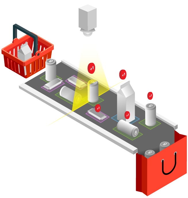
The software processes video stream in real-time, so after the product item crosses the counting line its quantity in the shopping bill is incremented. The average accuracy of our technology for instant checkout is 97% and is reaching 100% if the products are not touching while transported over the checkout conveyor.
Technologies behind Abto Cashier-less Checkout
- Computer vision
- Video & Image processing
- Robust feature extractors
- Deep learning
- Object recognition & counting
Benefits of Abto Computer Vision Powered Checkout
Our cashier-less technology allows both big supermarkets and small convenience stores provide their consumers with a seamless shopping experience without pausing the business operation for upgrading the checkout area. The benefits include:
- Fast and convenient in-store checkout
Customers can actually put items side-by-side and let them be counted all at once rather than have a cashier scan one item at a time. We can scan over 130 items in a minute and spare the customers the frustrations often encountered with traditional point-of-sales and self-checkouts. Therefore our approach ensures the growth of the store attendance, the checkout conversion rate, and the average shopping cart price that increases the overall store profit. - Responsive store management
Our solution allows switching between cashier operating mode and computer vision-assisted checkout-free mode. The manned checkouts may be optimized to handle exceptions, scan big items or new products while computer vision mode can free the staff to do more service-oriented tasks in the store. - Zero risks to consumers data privacy
Just Walk Out Technology employed by Amazon Go stores raises a lot of reasonable concerns regarding data protection. People are not always willing to give up their privacy in exchange for non-stop surveillance facilitating fast checkout. Moreover, most unmanned stores require customers to use their mobile apps in order to enter the store worsening the global tendency of smartphone addiction. Our technology helps businesses avoid those issues. Since our approach does not require customer identification it does not pose threats to consumers privacy and does not track their purchasing behavior. - Reduction of transaction time and operational costs
Our cashier-less technology allows your store to be always open, with the right staffing at the right time. It reduces losses from checkout shrink, attracts more customers and improves the overall retailer-customer relationship.
What’s next
- We have demonstrated how the PoC of our computer vision technology detects and counts five product classes. However, the product list is already extending. We are now able to distinguish and count very similar products within the same product line, say Snickers chocolate bars and Snickers with hazelnuts. The technology is now in the process of training on the new types of products. We are also experimenting with self-packed products like fruit, vegetables, and bread.
- We plan to develop our own API to integrate the cashier-less technology with the Point of Sale software for the supermarkets and grocery stores so the list of products can be automatically uploaded into the POS.